How Deep Learning Works

The field of Artificial Intelligence began to develop after World War II (the name was coined in 1956). But it wasn’t until the late 20th century that widespread applications began to emerge, with the first spam detectors and recommendation engines.

In the 2020s, the emergence of Generative Artificial Intelligence appears poised to revolutionize the way people interact with technology.

For end users, it allows them to “talk to the Internet” and ask questions or request services from systems that understand natural language and, most importantly, respond in kind.

For professionals, the possibility of AI taking over some of our jobs, even some of the most creative ones, represents a paradigm shift whose consequences will take decades to fully understand.

And for us software developers, AI is simply part of the ecosystem. It’s highly unlikely that a programmer starting their career in 2030 won’t have to work daily with Artificial Intelligence, whether it’s writing code, evaluating it, or requesting third-party services.

That’s why I consider it vital for any programmer to have at least a general understanding of how Artificial Intelligence works, just as you need to have knowledge of basic algorithms.

And both Artificial Neural Networks and Deep Learning are central concepts in AI.

In this article, I’ll cover everything you need to know to understand how Deep Learning works and program your own Neural Network.

The sample code is written in TypeScript because it’s an easy-to-understand language and can be programmed even within a web browser. Although in real life you’d never use this language to develop a model and deploy it to production due to poor performance, the important thing to learn is to use a language you’re comfortable programming in.

You can find the source code for this article in this GitHub repository.

As we’ll see, creating a Neural Network is relatively simple. But to understand how the training process works, you’ll need some knowledge of calculus. In particular, you’ll need some proficiency with:

Linear functions
Derivation and gradient
Vectors and Matrices

But don’t be scared, as long as you have a general understanding of the concepts, you don’t have to be a professional mathematician, far from it.

Disclaimer

The network we’re going to study is a model, a toy. I don’t write these things professionally, so many of the decisions I’ve made are certainly not optimal.

My goal is that, if you follow this article and use my code as an example to build your own model, you’ll learn as much as possible about how neural networks work. I followed myself this other article by Douglas Reiser as part of the preparation.

Think of the model we are going to build as a small training boat for children learning to sail: it works in its essentials, but you wouldn’t use it to cross the Pacific ;-)

Velero Ligero

Okay, let’s get to it.

1. What is Deep Learning?

Before getting into the nitty-gritty, it’s important to provide some context to understand exactly where we are. Let’s start with some definitions:

Artificial Intelligence (AI) is a branch of computer science that seeks to develop agents that simulate human reasoning.

Machine Learning (ML) is a branch of AI that seeks to generate software capable of training a model of reality from known data, to search for patterns and make predictions.

There are two main types of Machine Learning:

Supervised ML, in which the training data is labeled. For example, when you identify your family members’ faces in Google Photos so it can group all photos where they appear, you’re participating in the supervised learning process of an ML model.
Unsupervised ML, which works with unlabeled data to look for patterns or natural groups. For example, when Netflix suggests series “based on your preferences,” it’s using an unsupervised learning model that puts you in a group with other users who watch similar content, and recommends what they’ve liked.

Deep learning is a branch of machine learning that uses a type of model called “artificial neural networks”. The main advantage of these models over other types of machine learning is that they can identify (learn) more complex patterns.

“Generative Artificial Intelligences” such as Dall-E and “Large Language Models” (LLMs) such as ChatGPT or Google Bard are branches of Deep Learning.

In this article we will focus on understanding how neural networks and Supervised Machine Learning works, and finally how to program a Neural Network from scratch with TypeScript.

2. How does an Artificial Neural Network work?

Red Neuronal

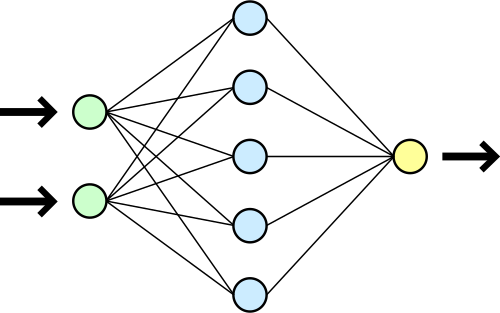
The idea behind neural networks is very simple. They are structures made up of nodes organized into layers. The basic principle of how they work is:

Each node executes a mathematical function that we call an “activation function,” which, for a given input, returns an output.
The first layer receives the input values, one for each node, and each node calculates its output value.
At each node in the second layer, the input is a weighted sum of the outputs of the nodes in the previous layer (i.e., each node’s output is multiplied by a weight, and all values are added up), plus an additional value called “bias”.
This process is repeated layer by layer until the network output is obtained, which is the result of the nodes that make up the last layer.

In mathematical language:

For each node of a particular layer we define

\begin{equation} a = f(z), \end{equation}

\begin{equation} z = w_0a_0 + w_1a_1 + \cdots + w_na_n + b \end{equation}

where

\(a\) is the result of the activation function
\(z\) is the sum of the activations of the nodes in the previous layer \(a_i\) multiplied by their weights \(w_i\), plus a bias \(b\).

What is the Activation Function?

One of the things to understand about neural networks, and machine learning in general, is that the concepts are simple, but there are a lot of decisions that don’t have a scientific explanation to justify them.

The activation function is an example of this. In principle, almost any function will do, but depending on what we’re using the neural network for, some work better than others.

It’s common for the activation function to be different for the input layer, the hidden layers, and the output layer. For simplicity, we’ll use a single activation function for now.

One of the most common choices is to use a sigmoid function, for example the logistic curve:

\begin{equation} f(z) = {1 \over (1 + e^{-z})} \end{equation}

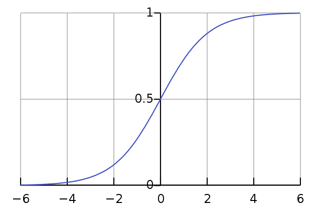Sigmoid Source: Wikipedia

This is a function that will always give a value between 0 and 1 for any value of \(z\). It is also a continuous and derivable, which is useful for training as we will see later.

What about the bias?

The bias value \(b\) we saw in the previous section is there to add a threshold to the weighted sum.

We can think of it as the value that the sum has to exceed so that \(z\) be positive, and therefore the activation function goes from values close to 0 to values close to 1.

3. Neural network code

The neural network is represented by the Network and Node classes:

export default class Network {

    private _input: number[] = [];

    constructor(
        readonly layers: Node[][],
        readonly activationFunction: ActivationFunction) { }

 ... 

    public calculate(input: number[]): number[] {
        this._input = Object.assign([], input);

        if (input.length !== this.layers[0].length) {
            throw (`Input size (${input.length}) doesn't match first layer size (${this.layers[0].length})`);
        }
        for (let layer of this.layers) {
            input = this.calculateLayer(input, layer);
        }

        this._output = input;
        return this._output;
    }

    private calculateLayer(input: number[], layer: Node[]): number[] {
        let result = []
        for (let node of layer) {
            result.push(node.calculate(input));
        }
        return result;
    }

    ...


export default class Node {
    private _zValue: number = 0;
    private _activation: number = 0;

...    
    calculate(input: number[]): number {
        this._zValue = this.calculateZValue(input);
        this._activation = this.activationFunction.calculate(this._zValue);
        return this._activation;
    }

    private calculateZValue(input: number[]): number {
        let sum = -1 * this.bias
        for (let i = 0; i < input.length; i++) {
            sum += this.weights[i] * input[i];
        }
        return sum;
    }
...

Essentially the Network class has a two-dimensional array of nodes and an activation function.

Whenever we want to calculate the output of the network, we iterate over the layers and for each layer we iterate over the nodes, asking each node to calculate its output value \(z\) and its activation value \(a\).

The output of the network is a vector the size of the last layer with the activations of its nodes.

To represent the activation function we create an abstract class that allows us to use different implementations:

export default abstract class ActivationFunction {
    abstract calculate(input: number): number;

    abstract calculateFirstDerivative(input: number): number;
}

As we can see, an activation function must be able to give us both the value for an input and the first derivative. We’ll see why when we talk about training.

The activation function we will use will be a sigmoid:

\begin{equation} f(z) = {1 \over (1 + e^{-z})} \end{equation}

\begin{equation} f’(z) = f(z)(1 - f(z)) \end{equation}

export default class SigmoidActivationFunction extends ActivationFunction {

    calculate(input: number): number {
        var output = (1 / (1 + Math.pow(Math.E, (-1) * input)));
        return output;
    }

    calculateFirstDerivative(input: number): number {
        const result = this.calculate(input);
        return result * (1 - result);
    }
}

The neural network is initially created with random weights and biases, using a Builder that allows us to set some of its characteristics:

const network = Network.builder([2, 5, 2]) // Three layers, of 2, 5 and 2 nodes
    .withWeightLimits(-1, 1) // with random weights between -1 and 1 (optional)
    .withBiasLimits(-1, 1) // with random bias values between -1 and 1 (optional)
    .withOutputProcessor(new NoOpFormatter()) // wighout output formatter (optional)
    .withActivationFunction(new SigmoidActivationFunction()) // with a sigmoid as activation function (optional)
    .build();

We will talk about the output processor later.

4. How is a neural network trained?

How does a child learn to distinguish a cow from a horse? A child doesn’t learn to distinguish every characteristic of each animal to make a real-time comparison between the two. Instead, they simply learn because people around them tell them “That’s a horse,” “That’s a cow.”

Well, a neural network learns the same way: we provide it with examples over and over again so that it can adjust its internal structure and be able to reproduce them.

The first thing we need to teach a neural network is a way to measure its error, so we can find ways to reduce it. We call cost function to the function that gives us the size of the error in a neural network’s prediction.

As with the activation function, we can choose from several options when selecting a cost function. One of the most common is the squared error:

\begin{equation} C(a) = {1 \over 2 }(a - o)^2 \end{equation}

Where \(a\) is the output of the neural network and \(o\) is the expected value. We take the square of \((a - o)\) so that it always gives us positive values, and we multiply it by \( 1 \over 2 \) so that the derivative will simply be:

\begin{equation} C’(a) = a - o \end{equation}

Once we have a way to calculate the error the network has made in a prediction, the training process becomes similar to an optimization problem. We will iteratively adjust the network’s weights and biases so that that error is as small as possible.

And to bring this into code we need to talk about two algorithms: Gradient Descend and BackPropagation

What is Gradient Descent?

The gradient descent algorithm is used to find the minimum of a function, in our case, the cost function.

The idea is as follows:

We start with a neural network initialized with random weights. Biases are typically initialized to zero.
We introduce a set of examples for which we know the expected result in advance.
We ask the network to calculate the output for each input value.
We calculate the value of the cost function for each result obtained.
We calculate the gradient of the cost function, which is the multivariate derivative of the function with respect to all the network parameters (the weights and biases).
We modify each weight by adding a value equal to the derivative of the cost function with respect to that particular weight, with the opposite sign, multiplied by a value we call the “learning rate,” which we’ll discuss later. We do the same with the biases.
We repeat steps 1 to 6 until the cost function no longer decreases.

Let’s take a closer look at the algorithm’s rationale.

As you may remember from your calculus studies, the derivative of a function (or the gradient if we’re talking about a vector field) gives us the slope of the function. If the function rises sharply at a specific point, the derivative evaluated at that point will have a large positive value. If, on the other hand, it drops downward, the value will be negative. And if the function is flat at that point, the derivative will be zero.

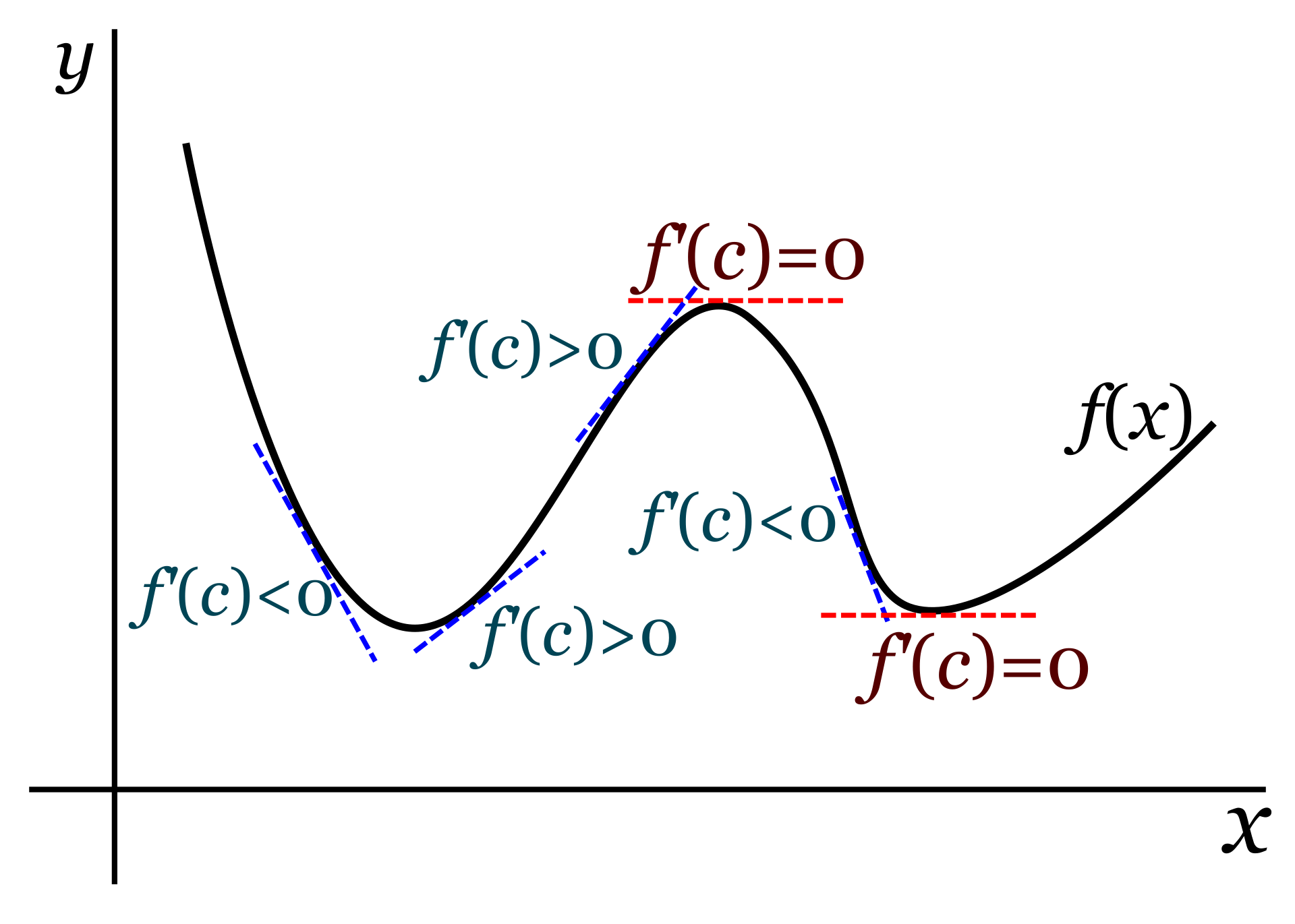Fermat’s Theorem Source: Wikipedia

Therefore, we identify a minimum of the function as a point for which the derivative is negative before that point, equals zero right at the point, and is positive right after.

The idea is that, if for a given value of weight \(w_i\), the derivative of the cost function with respect to that weight is negative, that means the function is declining at that point. Since we want to move toward the minimum of the function, we’ll need to try a larger value. However, if the derivative is positive, it means the function is increasing, and what we need is to move back to a smaller value of \(w_i\).

The learning rate would be the size of the jump we want to make when choosing the next value of \(w_i\). We need to choose this value carefully: if it’s too large, we may miss a minimum of the function. But if we choose it too small, learning may stagnate and we may never reach the minimum.

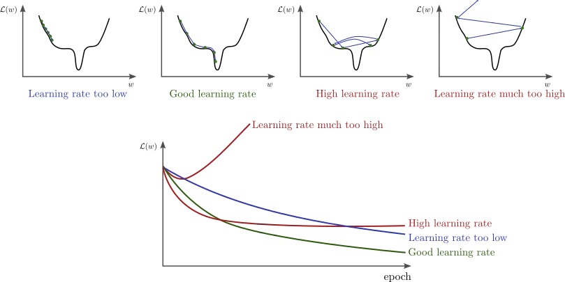Consequences of using learning rate values that are too large or too small Source: http://www.bdhammel.com/learning-rates/

Therefore, to train a neural network we “just” need to calculate the cost function, and its derivative with respect to the weights and biases, and try out values until we find the minimum.

Remember that, for a node in a particular layer, the cost \(C(a)\) is a function of its activation, but activation is a function of its z-value, which is a function of the weights, biases, and activations of the nodes in the previous layer.

Let’s call \(C_0\) the cost of the last layer (which measures the network’s error in predicting the outcome of an example input). In order to calculate the partial derivative of \(C_0\) with respect to the \(ij\)-th weight of the \(l\) layer we need to apply the chain rule:

\begin{align} \frac{\partial{C_0}}{\partial {{w_i}_j}^l} = \frac{\partial{z_j^l}}{\partial {{w_i}_j}^l} \frac{\partial{a_j^l}}{\partial z_j^l} \frac{\partial{C_0}}{\partial a_j^l} \end{align}

And we would do an analogous calculation to find the component corresponding to the bias \(b_i^l\).

And here we find two problems:

\(a_j^l\) is actually \(a_j^l({{w_i}_j}^{l-1}, a_j^{l-1}, b_j^{l-1})\): it depends on the weights, biases and activations of the previous layer.
Furthermore, the weights and biases can be tens, thousands, or millions of parameters, depending on the size of the network.

So calculating the derivative is by no means a trivial matter. Fortunately, it’s a well-studied problem and can be solved with the BackPropagation algorithm.

What is BackPropagation?

The BackPropagation algorithm allows you to efficiently calculate the gradient of the cost function. It involves traversing the network layers from the last layer backward, and for each layer, executing the following routine on all nodes:

If we are in the last layer, we calculate the derivative of the cost function with respect to the activation \(\frac{\partial{C_0}}{\partial a_i}\), and we keep the result in memory.
We calculate \(\frac{\partial{C_0}}{\partial b_i} = \frac{\partial{C_0}}{\partial a_i} \frac{\partial{a_i}}{\partial z_i} \frac{\partial{z_i}}{\partial b_i} \), knowing that \(\frac{\partial{z_i}}{\partial b_i} = 1 \).
For each weight \(w_i\) in the node:
- We calculate \(\frac{\partial{z_i}}{\partial w_i} \)
- Then we calculate \(\frac{\partial{C_0}}{\partial w_i} = \frac{\partial{C_0}}{\partial a_i} \frac{\partial{a_i}}{\partial z_i} \frac{\partial{z_i}}{\partial w_i} \) reusing the values from step 2.
- If we have not yet reached the first layer, we store the partial cost with respect to the activation of the previous layer \(a_i^l\): \(\frac{\partial{C_0}}{\partial {a_i}^l} = \frac{\partial{C_0}}{\partial a_i} \frac{\partial{a_i}}{\partial z_i} \frac{\partial{z_i}}{\partial a_i^l} \), where \(\frac{\partial{z_i}}{\partial a_i^l}\) is simply the weight \(w_i\) from that activity in the previous layer at this node. On the next turn of the loop, we’ll retrieve this value to construct the next gradient component.

It can be mathematically verified that this algorithm produces the same result as applying the chain rule.

Ok, let’s see the code now.

5. Code for the supervised learning process

Just like we did with the activation function, the cost function will be represented by classes extending an abstract class:

export default abstract class CostFunction {
    abstract calculate(actualResult: number, expectedResult: number): number;
    abstract calculateFirstDerivative(actualResult: number, expectedResult: number): number;

    private getCostArray(actualResult: number[], expectedResult: number[]): number[] {
        let cost: number[] = [];
        for (let i = 0; i < actualResult.length; i++) {
            cost.push(this.calculate(actualResult[i], expectedResult[i]));
        }
        return cost;
    }

    getTotalCost(actualResult: number[], expectedResult: number[]) {
        let costArray = this.getCostArray(actualResult, expectedResult);
        return costArray.reduce((a, b) => a + b);
    }
}

export default class QuadraticCostfunction extends CostFunction {

    calculate(actualResult: number, expectedResult: number): number {
        return Math.pow(actualResult - expectedResult, 2) / 2;
    }

    calculateFirstDerivative(actualResult: number, expectedResult: number): number {
        return actualResult - expectedResult;
    }
}

You can see the training process for example in this script:


const rounder = new OutputRounder();
const network = Network.builder([2, 2])
    .withWeightLimits(-1, 1)
    .withBiasLimits(0, 0)
    .withOutputProcessor(rounder)
    .build();
const epochs = 1000;
const batches = 1;
const output = new CliOutput();
const cost = new QuadraticCostfunction();
const learningRate = new LearningRate(0, 1);
const trainDataset: TrainDataItem[] = [];

trainDataset.push(new TrainDataItem([1, 0], [0, 1]));
trainDataset.push(new TrainDataItem([0, 1], [1, 0]));

const trainConfig = TrainConfig
    .builder(network, trainDataset)
    .withLearningRate(learningRate)
    .withEpochs(epochs)
    .withBatchCount(batches)
    .withCostFunction(cost)
    .withOutput(output)
    .withGainThreshold(0)
    .build();

const trainer = new Trainer(trainConfig);

const result = trainer.execute();

In this example we want to train the network to reverse the order of the input values: if we give it [1,0] it will return [0,1] and vice versa.

To do this, we start from an initial network with random biases and weights to which we add an output processor that rounds the values: in this way we ensure that we always have zeros or integer ones in the output, and we reduce the number of passes necessary on the training data, because as soon as the value found by the network is less than 0.5 it will be rounded to 0, and for larger values it will be 1.

We then create a training dataset, with objects of the TrainDataItem class that store an input value and the expected output value.

Next we define the training configuration using the TrainConfig class builder :

The LearningRate object allows us to define the increments of weights and biases in each training block.
The number of epochs, or times we are going to iterate through the test data.
The number of batches into which we want to divide the test data. For each batch, we will calculate the gradient of the cost function and modify the network weights and biases.
The gain threshold: when the improvement (in absolute value) in cost between two epochs does not exceed this value, we will stop training even if we have not yet reached the number of epochs.
Finally, we pass the training configuration to the Trainer to execute the learning process:


export default class Trainer {

    constructor(private config: TrainConfig) { }

    execute(): TrainResult {
        let t0 = Date.now();
        const result = new TrainResult();

        let lastCost = 0;
        for (let epoch = 0; epoch < this.config.epochs; epoch++) {

            const epochResult = this.executeEpoch(epoch);

            epochResult.calculateGain(lastCost);
            result.epochResults.push(epochResult);
            this.config.output.write(`Epoch #${epochResult.epochNumber} total cost: ${epochResult.cost} (${epochResult.costGainPercent}%)`);
            lastCost = epochResult.cost;

            if (Math.abs(epochResult.costGain) < this.config.gainThreshold) {
                this.config.output.write(`\nReached cost gain threshold. Interrupting.`);
                break;
            }
        }
        let t1 = Date.now();

        result.durationMs = t1 - t0;
        return result;
    }


    private executeEpoch(epoch: number): TrainEpochResult {
        let t0 = Date.now();
        const result = new TrainEpochResult(epoch);
        const batches = this.config.batches;
        for (let i = 0; i < batches.length; i++) {
            this.executeBatch(batches[i], result);
        }
        let t1 = Date.now();
        result.duration = t1 - t0;
        return result;
    }

    private executeBatch(items: TrainDataItem[], result: TrainEpochResult) {
        const network = this.config.network;
        const costFunction = this.config.costFunction;
        const tunner = new NetworkTunner(this.config.network, this.config.learningRate);
        for (let i = 0; i < items.length; i++) {
            const item = items[i];
            const output = network.calculate(item.input);
            const backProp = new BackPropagation(network, item.expectedOutput, costFunction);
            backProp.calculate(tunner);

            result.cost += backProp.totalCost;
        }
        tunner.apply(network);
    }

In each batch, the network output will be calculated for the included training elements, and the BackPropagation algorithm will be executed to parameterize the NetworkTunner that will calculate the changes to be made in weights and biases for the next batch.

export default class BackPropagation {

...

    calculate(tunner: NetworkTunner) {
        const layerCount = this.network.layers.length;
        for (let layerIndex = layerCount - 1; layerIndex >= 0; layerIndex--) {
            const layer = this.network.layers[layerIndex];
            for (let nodeIndex = 0; nodeIndex < layer.length; nodeIndex++) {
                const node = layer[nodeIndex];
                this.calculateForNode(node, tunner);
            }
        }
    }

    private calculateForNode(node: Node, tunner: NetworkTunner) {

        if (node.layer == this.network.layers.length - 1) {
            const actualResult = node.activation;
            const expectedResult = this.expectedResult[node.index];
            this._totalCost += this.costFunction.calculate(actualResult, expectedResult);

            const costRespectActivation = this.costFunction.calculateFirstDerivative(node.activation, expectedResult);
            this.saveCostRespectActivation(node.layer, node.index, costRespectActivation);
        }

        const zRespectBias = 1;
        const activityRespectZ = this.network.activationFunction.calculateFirstDerivative(node.zValue);
        const costRespectActivation = this._costRespectActivationCache[node.layer][node.index];
        const costRespectBias = costRespectActivation * activityRespectZ * zRespectBias;
        tunner.addGradientComponentBias(node.layer, node.index, costRespectBias);

        for (let w = 0; w < node.weights.length; w++) {
            const zRespectWeight = this.network.calculateDerivativeOfInputRespectWeight(node.layer, node.index, w);
            const costRespectWeight = costRespectActivation * activityRespectZ * zRespectWeight;
            tunner.addGradientComponentWeight(node.layer, node.index, w, costRespectWeight);
            if (node.layer > 0) {
                const zRespectPreviousActivation = this.network.calculateDerivativeOfZRespectPrevActivation(node.layer, node.index, w);
                const costRespectPreviousActivation = costRespectActivation * activityRespectZ * zRespectPreviousActivation;
                this.saveCostRespectActivation(node.layer - 1, w, costRespectPreviousActivation);
            }
        }
    }

export default class NetworkTunner {

...

    addGradientComponentBias(layerIndex: number, nodeIndex: number, value: number) {
        this._gradient[layerIndex][nodeIndex].bias += value;
    }

    addGradientComponentWeight(layerIndex: number, nodeIndex: number, weightIndex: number, value: number) {
        this._gradient[layerIndex][nodeIndex].weights[weightIndex] += value;
    }

    apply(network: Network) {
        for (let i = 0; i < network.layers.length; i++) {
            const layer = network.layers[i];
            for (let j = 0; j < layer.length; j++) {
                const node = layer[j];
                const deltas = this._gradient[i][j];
                this.applyNodeChanges(node, deltas);
            }
        }
    }

    private applyNodeChanges(node: Node, gradientComponents: GradientComponents) {
        const biasDiff = gradientComponents.bias * this.learningRate.biasLearningRate;
        node.bias -= biasDiff;
        for (let w = 0; w < node.weights.length; w++) {
            const weightDiff = gradientComponents.weights[w] * this.learningRate.weightsLearningRate;
            node.weights[w] -= weightDiff;
        }
    }
}

The TrainEpochResult class allows us to count the number of correct answers in each epoch and the gain (how much the cost decreases) between one epoch and the next:

export default class TrainEpochResult {

    duration: number = 0;
    cost: number = 0;
    costGain: number = 0;
    costGainPercent: number = 0;

    totalPredictions: number = 0;
    correctPredicitons: number = 0;

    constructor(readonly epochNumber: number) { }

    calculateGain(previousCost: number) {
        this.costGain = this.cost - previousCost;
        if (previousCost == 0) {
            return;
        }
        this.costGainPercent = Math.round(10000.0 * this.costGain / previousCost) / 100;
    }

    countResult(isCorrect: boolean) {
        this.totalPredictions++;
        if (isCorrect) {
            this.correctPredicitons++;
        }
    }

    get accuracy(): number { return Math.round(10000 * this.correctPredicitons / this.totalPredictions) / 100; }
}

The accuracy of our network will be the percentage of hits with respect to the total number of attempts.

The output of the example will be similar to this:

$ ts-node ./src/main.ts

Epoch #0 total cost: 0.599452087801611 (0%). Accuracy: 0% 
Epoch #1 total cost: 0.5901566456523485 (-1.55%). Accuracy: 0% 

...

Epoch #8 total cost: 0.5478469500940051 (-0.79%). Accuracy: 50% 
Epoch #9 total cost: 0.5437631943013445 (-0.75%). Accuracy: 50% 

...

Epoch #31 total cost: 0.42510398809990124 (-1.85%). Accuracy: 100% 
Epoch #32 total cost: 0.41691815979552177 (-1.93%). Accuracy: 100% 

...

Epoch #999 total cost: 0.10974016776822586 (0%). Accuracy: 100% 

Training complete. Average accuracy: 98.05%

If you try running the script several times, you will see that sometimes it will learn faster than others, and in some cases it will even complete all the epochs and will not achieve an accuracy greater than 50%.

Try changing the number of epochs, the ranges of weights and biases, or the number of layers and nodes, and you’ll see how the network’s learning capabilities change.

I also recommend using the debugger to follow step-by-step how values are calculated during training and understand the inner workings.

6. Conclusions

Well, that’s it! If you’ve understood everything up to this point, congratulations, because you now understand how neural networks work and are trained.

I hope this reading has been helpful in helping you understand this field a little better. I’ve tried to cover all the necessary concepts without going into too much depth so that the content can be followed relatively easily.

One of the main ideas I’d like to emphasize is that Artificial Intelligence is nothing more than mathematics. Quite simple concepts ingeniously applied to find patterns in reality and simulate human behavior.

And since mathematics is what it is, anyone can come to understand how it works.

7. References

I’ll leave you with some references that I’ve found especially useful for you to delve deeper into the topic:

Vídeos

Articles

Books

S. Russell y P. Norvig: “Artificial Intelligence, a modern approach” If you want to delve deeper into this field, I highly recommend this book where you will find practically everything there is to know about AI. There is a new edition available.