Efficient Vector Search
In my previous article, I presented VulcanoDB, an experiment to create a minimalistic, in-process vector database. Vector databases represent a critical component for AI-centric software, like retrieval-augmented generation, or agentic applications. They play a fundamental role in preserving the contextual structure via semantic search, ensuring that only relevant information is included in our interactions with Large Language Models.
VulcanoDB implements indexing and similarity search for applications with a flexible architecture and simple on-boarding. However, it was limited to in-memory data storage, and some characteristics of the initial implementation made the engine very inefficient.
For example, I used arrays of double to store the data. Double-precision numbers allow for greater precision and a wider range of values, at the cost of a bigger size (64-bit vs 32-bit of float). VulcanoDB is designed to handle vectors generated by embedding models, which typically generate 32-bit values, and we aim to be able to handle millions of these high-dimensional vectors, so changing from double to float is clearly justified here.
This is easy to fix with a simple search and replace.
The second cause of inefficiency is harder to fix. Similarity search is implemented with a brute-force algorithm that calculates cosine similarity between the query and every vector stored in the database. With a time complexity of O(n), this approach is clearly not escalable.
In this article I will explore the changes introduced to solve this limitation. The next release introduces a new data store that adds real data persistence, and uses HNSW indexes to ensure high performance in vector searches even with big data sets.
Let’s start by understanding this structures and how they work.
What is an HNSW Index
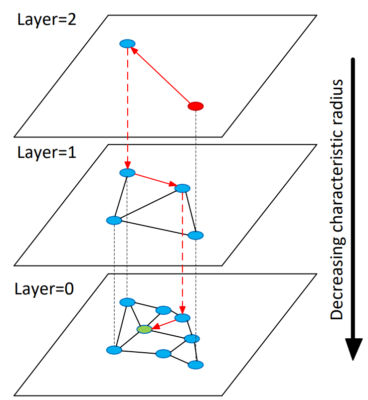
The Hierarchical Navigable Small World (HNSW) graph concept was introduced in 2016 by Yury A. Malkov and Dmitry A. Yashunin, in their paper “Efficient and robust approximate nearest neighbor search using Hierarchical Navigable Small World graphs ”. The authors propose a fully graph-based solution for Approximate Nearest Neighbor (ANN) search, that solves the problem of searching through massive datasets by organizing data into layers, which is conceptually similar to a Skip List, a probabilistic data structure that supports efficient search.
The typical analogy used to explain this algorithm is trying to find a specific street address in a massive country, where you divide the search by layers:
- Top Layer (Interstates): You start on a high-speed network with very few exits (long links). You move quickly toward the general vicinity.
- Middle Layer (Highways): Once you are close, you switch to a denser network to refine your location.
- Bottom Layer (Local Streets): Finally, you enter the local neighborhood (Layer 0) where every house is accessible, and you find the exact destination.
In an HNSW index, all elements reside in Layer 0 (the base layer), with progressively smaller random subsets occupying higher layers.
 Source: Image in the original paper
The Algorithms
The paper describes five different algorithms around the data structure:
- Insert
- Search within a layer
- Select neighbors (Simple)
- Select neighbors (Heuristic)
- K-Nearest-Neighbors Search
Let’s discuss them in detail.
Algorithm #1: Inserting Vectors to the Index
Input parameters:
q- the new vectorefConstruction- the size of the candidate list used when building connections during index construction.M- the number of connections to create per layerMmax- the maximum number of connections a vector can havemL- the highest layer a new vector can be added to
When adding a new vector q to the index:
- Randomly choose a maximum layer, using a function that produces smaller values with a higher probability than the bigger ones. The paper proposes something like this:
// - ThreadLocalRandom.current().nextDouble() is a double between 0.0 and 1.0
// - Since the logarithm of a number between 0 and 1 is negative, we change the sign
// - mL is an input parameter to the algorithm
//
// As a result, l is a random number between 0 and mL, but values close to 0
// are much more probable.
int l = (int) (-Math.log(ThreadLocalRandom.current().nextDouble()) * mL);
- Starting from the top layer, greedily find the closest vector to
qin that layer (see algorithm #2), then move down. Continue until you reach layerl. - From layer
ldown to 0:- Identify the
efConstructionnearest neighbors toq - Select the top
Mvectors from that group to connect toq. - If any of the selected vectors have more than
Mmaxconnections, remove part of them to maintain efficiency.
- Identify the
The result of this algorithm is that every vector is added to the layer 0, and to some of the higher layers (with lower probability as the layer index increases). Inside each layer, vectors are grouped by similarity.
Algorithm #2: Searching Within a Layer
Input parameters:
q- the new vectorep- the entry pointef- the number of nearest candidates (neighbors) to explorelc- the layer number
This algorithm is a Greedy Graph Search that operates within a single, specified layer of the HNSW structure. Its goal is to find the elements in the given layer that are closest to the query vector q.
We maintain three collections of vectors:
V- a set of visited vectorsC- a queue of candidates, ordered by their distance toqW- a list of results
Firstly, we add the entry point to the three lists. The search continues as long as there are candidates in C:
- Select and remove from
Cthe candidate that is closest toq,e. - If the distance from
eto the current best candidate is greater than the distance to the furthest element already inWthen the loop terminates. The logic behind this is that, sinceCis ordered by distance, the remaining elements will be even further away thaneand no further exploration can improve the current set of resultsW. - Explore the neighbors (see algorithms #3,#4) of
ein the current layer that have not been already visited. For each neighbore':- Add
e'toV - Calculate the distance from
qtoe' - If
e'is closer toqthan the furthest element inW, OR ifWhas not yet reached its maximumb sizeef:- Add
e'toW - If the size of
Wis now greater thanef, remove the furthest element.
- Add
- Add
e'toCfor future exploration.
- Add
When the loop terminates, the algorithm returns W, containing the ef nearest vectors to q in the lc layer.
Algorithms #3 and #4: Selecting Neighbors
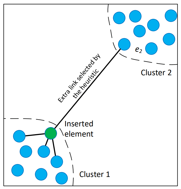
The paper describes two possible algorithms to select neighbors of a given vector within a layer. The simplest one is to use the distance function to pick the closest ones, that is Algorithm #3. But the authors propose using a heuristic to “significantly increase performance at high recall and in case of highly clustered data”.
 Source: Image in the original paper
This is how the heuristic works:
- When connecting the vector
qto candidates, the algorithm iterates through candidates from closest to furthest. - It connects a candidate
Ctoqonly ifCis closer toqthan it is to any already connected neighborR. - This creates a “Relative Neighborhood Map”, which maintains global connectivity even in highly clustered data, preventing the search grom getting stuck in a local cluster.
Now we have all the pieces to review the main algorithm.
Algorithm #5: Searching the K Nearest Neighbors from the index
Input parameters:
qthe query vector.Kthe number of neighbors to return.efthe search query parameter.
The final search method is a multi-stage process that leverages the layered graph structure to achieve logarithmic complexity scaling. It transitions from a coarse, high-speed “zoom-in” phase to a fine-grained, high-recall search at the ground layer.
- Upper layer “zoom-in” phase:
- The search starts at the highest layer (
L) - For every layer from
Lto to layer 1, perform a greedy search:- Invoke the layer search with
ef=1. - In every search, explore neighbors to find the closest element to the query
q. - This element becomes the entry point for the next layer down.
- Invoke the layer search with
- This phase then navigates the “espress lines” to quickly find the vecinity of the query without calculating many distances.
- The search starts at the highest layer (
- Ground layer fine search:
- Using the entry point from the previous layer, invoke the layer search with the configured value of
ef. - Mantain a dynamic list
Wof theefclosest found elements. It explores the neighbors of best candidates, updatingWas closer elements are found. - Stopping condition: the algorithm stops when the closest neighbor of the current base node is further from the query than the furthest element in the result
W.
- Using the entry point from the previous layer, invoke the layer search with the configured value of
- The returned result will be the
Kclosest elements toqfromW.
Because each layer requires only a near-constant number of steps, the overall search complexity grows logarithmically (O(log N)), where N is the number of vectors in the dataset.
The quality of the search (recall) is directly controller by ef. Increasing the value improves the probability of finding the true nearest neighbors at the cost of increasing the number of distance computations.
HNSW Index Implementation
The paper describes in great detail the data structure, and the algorithms used to insert and search vectors. But there are many things left as implementation details, so building this index implies making some decissions. Let’s discuss the main ones.
Distance metric
The whole paper uses the distance between vectors as the key metric. However, in this implementation I use cosine similarity to compare vectors, consistent with the original design of VulcanoDB. This causes all the comparisons to reverse (small distance vs big similarity).
Memory scaling strategy
To model the HNSW graph, we could use a fully object-oriented approach, creating a Node class that would contain a vector and its neighbors, and then model the layers as Lists of such objects. But the whole point of this project is to have a high performant, highly scalable structure, and standard Java objects carry significant hidden costs, specifically object headers (12-16 bytes per object) and pointer references (4-8 bytes). When you scale to millions of nodes, this overhead can easily consume more RAM than the actual vector data itself, triggering frequent Garbage Collection (GC) pauses that kill search performance.
The paper highlights that their C++ implementation uses “custom distance functions together with C-style memory management” to avoid overhead and allow hardware prefetching. To achieve similar efficiency in Java, we must abandon standard OOP practices in favor of primitive arrays and flattened memory layouts.
Vector storage (layer 0)
For layer 0, that contains every vector in the index, it would make more sense to store all the vectors in a flat array and then work with offsets to access to them. The problem with this is that due to arrays using integer indices, we would be limited to ~2.1 billion elements, or ~2GB of total data.
To avoid this limitation, we use Project Panama’s MemorySegment class, which allocates “off-heap” memory that behaves like a C++ array. The PagedVectorIndex class models a vector index that uses paging to scale:
final class PagedVectorIndex {
    // List of memory segments (pages)
    private final List<MemorySegment> pages = new ArrayList<>();
    private final AtomicLong currentCount = new AtomicLong(0);
    private final int blockSize;
    private final int dimensions;

    /**
     * @param blockSize  how many vectors per page
     * @param dimensions how many elements per vector
     */
    public PagedVectorIndex(int blockSize, int dimensions) {
        this.blockSize = blockSize;
        this.dimensions = dimensions;

        if (blockSize < 1) {
            throw new IllegalArgumentException("Invalid block size, must be > 0");
        }
        if (dimensions < 1) {
            throw new IllegalArgumentException("Invalid dimensions, must be > 0");
        }
        // Start with one page
        addPage();
    }

    private void addPage() {
        // Allocate off-heap memory for 1 block of vectors
        long byteSize = (long) blockSize * dimensions * Float.BYTES;
        MemorySegment newPage = Arena.ofAuto().allocate(byteSize);
        pages.add(newPage);
    }

    //... other class members
}
We need to fix the number of dimensions so that all the vectors have the same size.
Using an AtomicLong to store the internal offset ensures that the data structure is thread safe. The method to add new vectors to this structure will create new pages automatically as required:
public long addVector(float[] vector) {
    long internalId = currentCount.getAndIncrement(); // Atomic, gives unique ID

    // 1. Check if we need a new page
    if (internalId % blockSize == 0 && internalId > 0) {
        // Synchronize only the slow, array-modifying operation
        synchronized (this) {
            // Double-check lock: check again in case another thread already added the page
            if (pages.size() <= internalId / blockSize) {
                addPage();
            }
        }
    }

    // 2. Calculate location
    int pageIdx = (int) (internalId / blockSize);
    long offset = (internalId % blockSize) * dimensions * Float.BYTES;

    // 3. Write data (MemorySegment is generally thread-safe for disjoint writes)
    MemorySegment.copy(vector, 0, pages.get(pageIdx), ValueLayout.JAVA_FLOAT, offset, dimensions);

    return internalId;
}
Then, to retrieve a vector by its offset, we only need to determine the page and read from the MemorySegment:
public float[] getVector(long id) {
    if (id < 0 || id >= currentCount.get()) {
        throw new IllegalArgumentException("Illegal vector id");
    }
    int pageIdx = (int) (id / blockSize);
    long pageOffset = (id % blockSize) * dimensions * Float.BYTES;
    var sliceSize = dimensions * Float.BYTES;

    var slice = pages.get(pageIdx).asSlice(pageOffset, sliceSize);
    return slice.toArray(ValueLayout.JAVA_FLOAT);
}
Connection storage
Once we have the structure to allocate the vectors, we need the one that will store the connections. Instead of storing a List<List<Integer>> (which creates millions of small objects), we will pre-allocate a fixed “slot” of memory for every node’s connections (Flattened Adjacency List).
Visually:
[ Node 0 Data ........................ ] [ Node 1 Data ........................ ]
| Count (int) | N1 | N2 | ... | N_max |  | Count (int) | N1 | N2 | ... | N_max |
The PagedGraphIndex class uses a similar strategy as PagedVectorIndex:
final public class PagedGraphIndex {
    // Max neighbors for Layer 0 (usually 2 * M)
    private final int maxConnections;

    // Size of one node's connection data in bytes:
    // 4 bytes (count) + (mMax0 * 8 bytes)
    private final int slotSizeBytes;

    private final int blockSize; // Nodes per page
    private final List<MemorySegment> pages = new ArrayList<>();

    public PagedGraphIndex(int maxConnections, int blockSize) {
        this.maxConnections = maxConnections;
        this.slotSizeBytes = Integer.BYTES + (maxConnections * Long.BYTES);
        this.blockSize = blockSize;
        addPage();
    }

    private void addPage() {
        long totalBytes = (long) blockSize * slotSizeBytes;
        pages.add(Arena.ofAuto().allocate(totalBytes));
    }

    private void ensureCapacity(long vectorId) {
        int pageIdx = (int) (vectorId / blockSize);
        while (pages.size() <= pageIdx) {
            addPage();
        }
    }

    /**
     * Overwrites the connections for a specific node.
     * Used after the Heuristic (Algorithm 4) selects the best neighbors.
     */
    public void setConnections(long vectorId, long[] neighbors) {
        if (neighbors.length > maxConnections) {
            throw new IllegalArgumentException("Too many neighbors");
        }
        ensureCapacity(vectorId);

        // 1. Calculate Offsets
        int pageIdx = (int) (vectorId / blockSize);
        long pageStart = (vectorId % blockSize) * slotSizeBytes;
        MemorySegment page = pages.get(pageIdx);

        // 2. Write Count
        page.set(ValueLayout.JAVA_INT, pageStart, neighbors.length);

        // 3. Write Neighbors
        // We skip 4 bytes (the count) to find the start of the neighbor array
        long neighborArrayOffset = pageStart + Integer.BYTES;

        MemorySegment.copy(
                MemorySegment.ofArray(neighbors), 0,
                page, neighborArrayOffset,
                (long) neighbors.length * Long.BYTES
        );
    }
    // ... other class members ...

}
The HnswIndex class
The HnswIndex class implements the main management algorithms described in the paper, delegating the data storage to the previously discussed PagedVectorIndex and PagedGraphIndex classes:
public class HnswIndex {
    private final HnswConfig config;
    private final PagedVectorIndex layer0;
    private final PagedGraphIndex layer0Connections;

    /*
    Only ~5% of the nodes exist in Layer 1, and ~0.25% in Layer 2. The memory overhead of Java objects here is
    negligible compared to the massive Layer 0.
     */
    private final Map<Integer, Map<Long, Set<Long>>> upperLayerConnections = new HashMap<>();

    private int globalMaxLayer = 0;
    private long globalEnterPoint = 0;

    public HnswIndex(HnswConfig config) {
        this.config = config;
        layer0 = new PagedVectorIndex(config.blockSize(), config.dimensions());
        layer0Connections = new PagedGraphIndex(config.mMax0(), config.blockSize());
    }

    //... other class members ...
}
The insert method adds a new vector to the index and returns the offset where it is stored:
public long insert(float[] newVector) {
    if (newVector.length != config.dimensions()) {
        throw new IllegalArgumentException(
                "Invalid vector dimension: %d (expected %d)".formatted(newVector.length, config.dimensions()));
    }

    long currentId = globalEnterPoint;
    int maxL = globalMaxLayer;

    //1. Randomly choose a maximum layer
    int vectorMaxLayer = determineMaxLayer();

    //2. Add vector to layer 0
    long newId = layer0.addVector(newVector);

    //3. Zoom down from Top Layer to vectorMaxLayer+1 (Greedy search, ef=1)
    for (int l = globalMaxLayer; l > vectorMaxLayer; l--) {
        currentId = searchLayerGreedy(newVector, currentId, l);
    }

    // 4. From L down to 0, find neighbors and link
    for (int layer = Math.min(vectorMaxLayer, maxL); layer >= 0; layer--) {
        // Search layer with efConstruction
        var neighborCandidates = searchLayer(newVector, currentId, layer, config.efConstruction());

        if (neighborCandidates.isEmpty()) {
            continue;
        }

        // Update entry point for next layer
        currentId = neighborCandidates.peek().vectorId(); // Rough logic, usually closest

        // Select neighbors using heuristic
        var neighbors = selectNeighborsHeuristic(neighborCandidates);

        // Add connections bidirectional
        for (long neighborId : neighbors) {
            // Register connection bidirectionally. Not both connections are guaranteed to be stored,
            // as there will be a pruning process for each node.
            addConnection(newId, neighborId, layer);
            addConnection(neighborId, newId, layer);
        }
    }

    // 5. Update global entry point if new node is in a higher layer
    if (vectorMaxLayer > globalMaxLayer) {
        globalMaxLayer = vectorMaxLayer;
        globalEnterPoint = newId;
    }
    return newId;
}
The search method implements the search algorithm:
/**
 * Returns the K-Nearest Neighbors of queryVector
 *
 * @param queryVector the physical vector
 * @param k           the number of vectors to return
 * @return a list of {@link NodeSimilarity} instances representing the search results.
 */
public List<NodeSimilarity> search(float[] queryVector, int k) {
    if (layer0.getVectorCount() == 0) {
        return Collections.emptyList();
    }

    long currObj = globalEnterPoint;

    // 1. Zoom-in Phase: Fast greedy search through upper layers
    // We use ef=1 for speed as we just need a good entry point for the next layer
    for (int l = globalMaxLayer; l >= 1; l--) {
        currObj = searchLayerGreedy(queryVector, currObj, l);
    }

    // 2. Fine Search Phase: Comprehensive search at the ground layer (Layer 0)
    // W is a Max-Heap that keeps track of the 'ef' best candidates
    PriorityQueue<NodeSimilarity> w = searchLayer(queryVector, currObj, 0, config.efSearch());

    // 3. Return top K results from the candidates found in Layer 0
    List<NodeSimilarity> results = new ArrayList<>();
    // W is a max-heap; we want the closest K, so we might need to sort or poll
    while (w.size() > k) {
        var o = w.poll(); // Remove furthest until we have K
    }
    while (!w.isEmpty()) {
        results.add(w.poll());
    }
    Collections.reverse(results);
    return results;
}
Performance Comparison
To evaluate the performance gain that this index introduces, I have created a sample application that compares the time taken to search on an indexed field against a non indexed one.
The example class creates a VulcanoDb instance, configured to index the indexedVector field:
    private static VulcanoDb createVulcanoDB() {
        var properties = new Properties();
        properties.setProperty(ConfigProperties.PROPERTY_PATH, path.toString());
        var hnswConfig = HnswConfig.builder()
                .withEfConstruction(500) // max recall
                .withEfSearch(500) // max recall
                .build();
        var axon = AxonDataStore
                .builder()
                .withDocumentWriter(new DefaultDocumentPersister(new TypedProperties(properties)))
                .withVectorIndex("indexedVector", hnswConfig)
                .build();

        return VulcanoDb
                .builder()
                .withDataStore(axon)
                .build();
    }
Then, a series of example texts are stored, creating the embedding for the text and adding it twice, once in the indexed field and the other in a non-indexed one:
    private static List<Document> generateSamples() throws URISyntaxException, IOException {
        var loader = Thread.currentThread().getContextClassLoader();
        var url = loader.getResource("rotten-tomatoes-reviews.txt");
        Path path = Paths.get(url.toURI());
        try (var lines = Files.lines(path)) {
            return lines
                    .parallel()
                    .map(txt -> {
                        var embedding = Embedding.of(txt);
                        return Document.builder()
                                .withStringField("originalText", txt)
                                .withVectorField("nonIndexedVector", embedding)
                                .withVectorField("indexedVector", embedding)
                                .build();
                    })
                    .toList();
        }
    }
The generated texts are stored, and then two queries are evaluated, searching for the same text both in the indexed and the non-indexed field to compare the time of each one:
...
IO.println("Generating embedding for the query...");
var query = "Clever horror movie with great acting";
var queryVector = Embedding.of(query);

IO.println("Non-indexed search:");
long t0 = System.currentTimeMillis();
var nonIndexedQuery = Query.builder().isSimilarTo(queryVector, "nonIndexedVector").build();
vulcanoDB
        .search(nonIndexedQuery, 10)
        .getDocuments()
        .forEach(HnswIndexPerformance::showResult);

long bruteTime = System.currentTimeMillis() - t0;
IO.println("Non-indexed search time: %d ms".formatted(bruteTime));


IO.println("Index search: ");
t0 = System.currentTimeMillis();
var indexedQuery = Query.builder().isSimilarTo(queryVector, "indexedVector").build();
vulcanoDB
        .search(indexedQuery, 10)
        .getDocuments()
        .forEach(HnswIndexPerformance::showResult);
var indexTime = System.currentTimeMillis() - t0;
IO.println("Index search time: %d ms.".formatted(indexTime));
The output of this example will be similar to the following:
Generating embedding for the query...
Non-indexed search:
[0.83] b0089fc7-ab3c-4b85-8daf-7d422a9f9567 -> a slick , skillful little horror film .
[0.80] 39a5e68b-171d-45f3-a3fa-8a9354512dba -> one of the best silly horror movies of recent memory , with some real shocks in store for unwary viewers .
[0.79] e4bcf721-412a-4392-8919-5e3a551d51f9 -> this is a superior horror flick .
[0.77] 6416021c-c35e-4c90-8f2e-8092ca1c7ba3 -> an exceedingly clever piece of cinema . another great ‘what you don't see' is much more terrifying than what you do see thriller , coupled with some arresting effects , incandescent tones and stupendous performances
[0.77] 0783c1fb-8719-40d5-a211-bead28e9a228 -> clever , brutal and strangely soulful movie .
[0.77] 414227e8-e428-494c-8bbd-9ef9608d9fb7 -> a chilling movie without oppressive gore .
[0.74] a8b28cb8-4884-46b1-9a58-f910286ab829 -> marshall puts a suspenseful spin on standard horror flick formula .
[0.74] c90ecce2-72e4-4321-9436-af5657dd3558 -> the entire movie establishes a wonderfully creepy mood .
[0.73] e95c46b6-4e44-4fa8-894b-1d595bc7ed2e -> a deftly entertaining film , smartly played and smartly directed .
[0.73] 449979ab-56ef-45b0-befc-4062f0ca68e6 -> if nothing else , this movie introduces a promising , unusual kind of psychological horror .
Non-indexed search time: 372 ms
Index search:
[0.87] 39a5e68b-171d-45f3-a3fa-8a9354512dba -> one of the best silly horror movies of recent memory , with some real shocks in store for unwary viewers .
[0.86] e4bcf721-412a-4392-8919-5e3a551d51f9 -> this is a superior horror flick .
[0.84] 0783c1fb-8719-40d5-a211-bead28e9a228 -> clever , brutal and strangely soulful movie .
[0.83] a8b28cb8-4884-46b1-9a58-f910286ab829 -> marshall puts a suspenseful spin on standard horror flick formula .
[0.83] c90ecce2-72e4-4321-9436-af5657dd3558 -> the entire movie establishes a wonderfully creepy mood .
[0.82] e95c46b6-4e44-4fa8-894b-1d595bc7ed2e -> a deftly entertaining film , smartly played and smartly directed .
[0.82] 65105ae3-32fd-449a-b0ec-414a8d487abf -> my little eye is the best little " horror " movie i've seen in years .
[0.81] e8635913-5f1f-474c-9ad2-9a46ea725483 -> a properly spooky film about the power of spirits to influence us whether we believe in them or not .
[0.81] d0a79c1c-cd0b-41f1-b48b-afdca5121811 -> an elegant film with often surprising twists and an intermingling of naiveté and sophistication .
[0.81] 190ea188-c21e-4def-be0f-822b47b97b18 -> a perceptive , good-natured movie .
Index search time: 22 ms.
This example illustrates two key observations:
- Querying on an indexed field is ~17 times faster. Not only that, it scales much better (O(log(N)) vs O(N)).
- The results are not exactly the same. Using a HNSW index means moving away from exact results, to an approximate K-Nearest neighbor search, which has to be taken into account.
Conclusion
I am on a journey to learn about modern AI tools and the principles that underpin them. Years ago I wrote about Deep Learning and built a simple artificial neural network in Typescript, to understand how these models are trained and how gradient descend algorithm works. More recently, I wrote about retrieval-augmented generation and built a multi-agent system to introduce myself to LLMs and how they are used to power different types of applications.
Then I focused on semantic search — a topic that has always resonated with me because it connects back to my physics background, much like the gradient-descent technique. I built VulcanoDb to understand the problems that vector databases solve and some of their solutions.
This article examined how real vector databases achieve efficient search using Hierarchical Navigable Small World (HNSW) indexes.
Thanks for reading!